I created a TED talk recommender using Natural Language Processing (NLP). See part1, for the initial exploration of the data and cleaning. This post will describe the different topic modeling methods I tried and how I used t-distributed Stochastic Neighbor Embedding (tSNE) to visualize the topic space. In Part 3, I post the actual recommender I created using flask. The code is available in my github.
Now that we have cleaned and vectorized our data, we can move on to topic modeling. A topic is just a group of words that tend to show up together throughout the corpus of documents. The model that worked best for me was Latent Dirichlet Allocation (LDA) which creates a latent space where documents that have similar topics are closer together. This is because documents from a similar topic tend to have similar words, and LDA picks up on this. We then assign a label to each topic based on the 20 most frequent words for each topic. This is where NLP can be tricky, because you have to decide whether the topics make sense or not, given your corpus of documents and model(s) that you have used.
A more detailed explanation of this process is that LDA will provide a (strength) score for each topic for each document, then I just assigned the strongest topic to each document. The other thing about LDA is that it will also yield a 'junk' topic (hopefully there's only one...) that won't make much sense, that's fine. It's putting all of the words without a group (they don't tend to show up with other words) into that topic. Depending on how much you clean your data, this can be tricky to recognize. When my data was still pretty dirty, it was where all of the less meaningful words would end up (i.e., stuff, guy, yo).
First get the cleaned_talks from the previous step. Then import the model with sklearn
from sklearn.decomposition import LatentDirichletAllocation
I put the model into a function along with the vectorizers so that I could easily manipulate the parameters like 'number of topics, number of iterations (max_iter), n-gram size (ngram_min, ngram_max), number of features (max_df). We can tune the hyperparameters to see which one gives us the best topics (ones that make sense to you).
The functions will print the topics and the most frequent 20 words in each topic. Here are a few examples from the TED Talks.
At this point try to put a name with each topic. For example, I called Topic 3 'marine biology' but you might call it 'environment'. Now that we have topics, we can assign the strongest topic to each document and create a dataframe of labels for our next step.
Then we create the dataframe with our custom labels
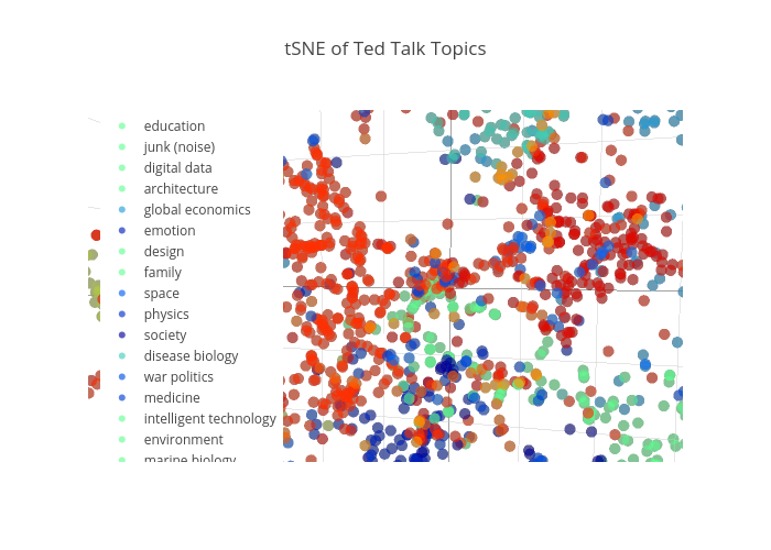
If we want to view this topic space to further check whether our modeling worked like we wanted it to, we can use tSNE. t-Distributed Stochastic Neighbor Embedding (tSNE) is a recent technique for reducing the dimensionality of a high-dimensional space, so that we can view it.
We humans suck at visualizing 20-dimensions, as you know. Once we plot our t-SNE we want to look for clusters. This means that the points (documents) that belong to the same topic are close together rather than spread out. I have code to plot it in matplotlib, but I prefer to use the one in plotly. Each point is a document (talk) and each color is a different topic, so points of the same color should be close together if our topic modeling is working. If they are spread out, it means that the documents in that particular topic are not very similar (which may not be the worst thing in the world, depending on what you are trying to do). I was not able to get a better color bar, so it is easier to view if you just isolate some of the topics rather than try to view all 20. You can do this by clicking on the topics in the legend. (see the 3D graph at the top of this page)
In Part 3, I post the actual recommender I created using flask.